4 A First Learned Classifier: Logistic Regression
How does a classifier learn its weights — and what exactly does it get right and wrong?
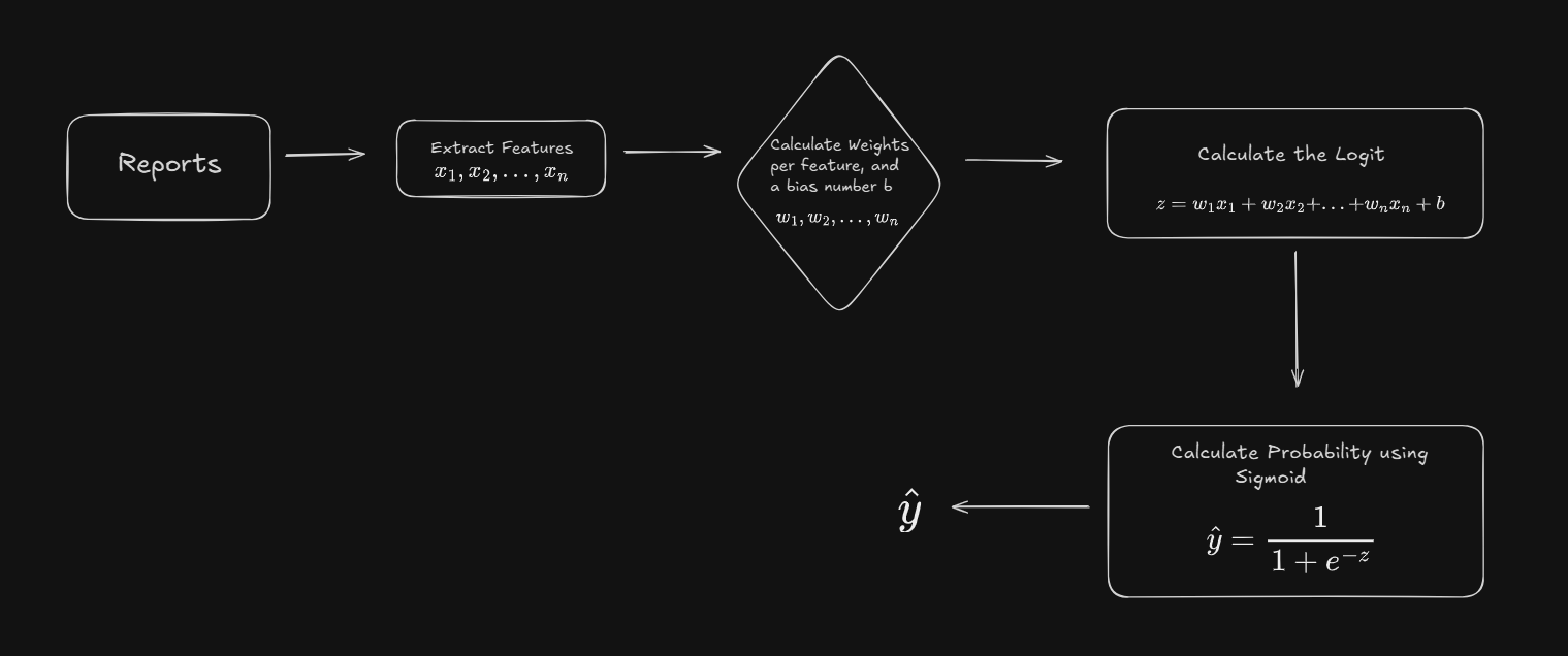
Two chapters have prepared the ground. Section 1.4.2 introduced logistic regression on toy data: a weighted sum of features, the logit \(z\), turned into a probability by the sigmoid, with weights we chose by hand.
Chapter 2 set up honest evaluation on the real reports: training, validation and test sets, a majority-class baseline, and a warning about leakage. It also met the limits of a method that learns nothing: nearest neighbors reached 87% by copying the labels of similar reports, mostly by recognizing each hospital’s template, and fell to 41% on hospitals it had never seen. So from here on, every split keeps each hospital’s reports in one pile, as the scoreboard of Section 3.6 did, and every score in this chapter is about hospitals the model has never seen. Chapter 3 also looked closely at how a report is split into words. This chapter keeps CountVectorizer’s standard splitting for logistic regression, and compares it with nearest neighbors at its best on new hospitals.
This chapter fills the gap Section 1.4.2 left — how the weights are learned — and then puts the learned classifier to work on the split by hospital, measures it in more detail than accuracy alone can, reads what it learned, and compares it with nearest neighbors.
Cells run in your browser and share one session, so run them in order from the top. The first one takes fifteen to thirty seconds while Python loads.
4.1 How the weights are learned
4.1.1 Back to the four reviews
Section 1.4.2 built a tiny problem: four product reviews, two positive and two negative, each described by four hand-made features — positive words, negative words, whether no appears, and the logarithm of the length. This cell rebuilds it, together with the logit and the sigmoid:
Each review gets two numbers. The logit \(z = \mathbf{w}\cdot\mathbf{x} + b\) can be any number. The sigmoid turns it into \(\hat{y} = \sigma(z)\), a probability between 0 and 1: the model’s estimate that the review is positive. The model says positive when \(\hat{y} > 0.5\).
All four are right, review 1 only narrowly. But we chose those weights. To learn them, the computer needs two things: a way to score a set of weights, and a way to improve them.
4.1.2 Cross-entropy loss: how wrong is a prediction?
A score for how good a set of weights is is called a loss: small when predictions are right, large when they are wrong.
Accuracy will not do. It only asks whether \(\hat{y}\) landed on the correct side of \(0.5\), so it cannot tell a lucky \(0.51\) from a confident \(0.99\), and it gives no hint about which way to nudge a weight.
The right loss asks: what probability did the model give to the answer that actually happened? For a true label of 1 that is \(\hat{y}\); for a true label of 0 it is \(1-\hat{y}\). Both cases fold into one expression:
\[ L(\hat{y}, y) = -\Big[\, y\log \hat{y} + (1-y)\log(1-\hat{y}) \,\Big]. \]
Because \(y\) is 0 or 1, one of the two terms always vanishes: when \(y=1\) the loss is \(-\log\hat{y}\), and when \(y=0\) it is \(-\log(1-\hat{y})\). This is the cross-entropy loss. It is \(0\) when the model puts probability 1 on the truth, and grows without limit as the model becomes confidently wrong. For review 1, with \(y^{(1)}=1\) and \(\hat{y}^{(1)}=0.7113\):
\[ L^{(1)} = -\log(0.7113) = 0.3407 . \]
Review 1 carries almost all of it: 0.34, against 0.01 or less for the others. All four predictions are correct, yet the loss is not zero, because being right by a narrow margin still counts against the weights. That is exactly what accuracy cannot see, and why the loss is the quantity to make as small as possible.
The widget below draws the loss for every possible \(\hat{y}\). Choose the true label, slide the prediction, or load one of the four reviews. The dashed line is all that accuracy sees: 0 on the correct side of 0.5, 1 on the wrong side, and flat everywhere else, so it cannot say which way to move. The loss keeps falling as the prediction grows more confident in the truth, and climbs steeply as it grows confident in the wrong answer: for a true label of 1, a prediction of 0.01 already costs 4.6.
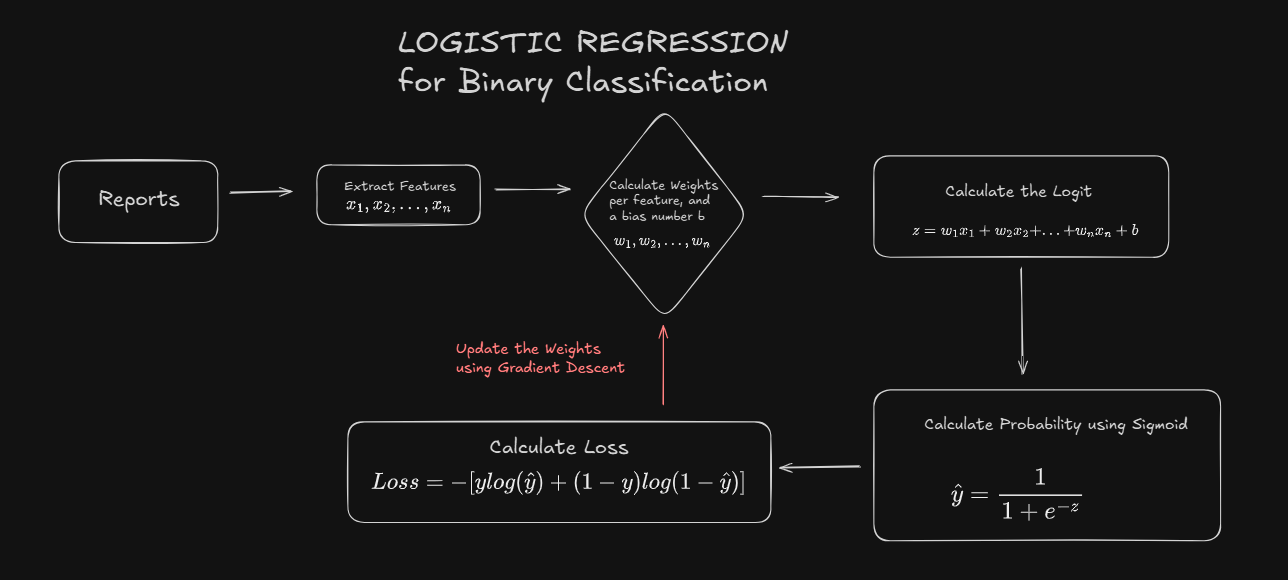
Here is the whole process so far. The red arrow is the step still missing: using the loss to improve the weights.
4.1.3 Gradient descent: how the weights are improved
Learning means searching for the weights that make the average loss as small as possible — and the loss itself says which way to go. For cross-entropy over a sigmoid, the slope of the loss with respect to each weight (its gradient) works out to something strikingly simple (Section C.1 derives it with the chain rule):
\[ \frac{\partial L}{\partial w_j} = (\hat{y} - y)\, x_j , \qquad \frac{\partial L}{\partial b} = (\hat{y} - y). \]
In words: the gradient for a weight is the prediction error times that feature’s value. If the prediction is right, \(\hat{y}-y\) is near zero and the weight barely moves. If it is confidently wrong, the error is close to \(\pm 1\) and every weight moves in proportion to how strongly its feature was present.
Stochastic gradient descent turns that into a procedure. Starting from some weights — say, all zero — repeat many times:
- take one training example, in random order (the stochastic part);
- compute \(z\), then \(\hat{y} = \sigma(z)\);
- compute the error \(\hat{y} - y\);
- nudge every weight and the bias against its gradient: \[ w_j \leftarrow w_j - \eta\,(\hat{y}-y)\,x_j , \qquad b \leftarrow b - \eta\,(\hat{y}-y). \] The bias has no feature value to multiply by, so it moves by the error alone.
The learning rate \(\eta\) sets the size of each step: too small and the search crawls, too large and it overshoots. One pass through all the training examples is an epoch. Here it is, running on the four reviews from all-zero weights:
Watch three things. The loss falls fast — from 0.55 after one epoch to 0.002 after a thousand. The weights for positive and negative words grow in the directions we expected. And the other two weights do not match our hunches from Section 1.4.2: the weight for no comes out positive, not negative, because no appears in one positive review and one negative one, and four examples cannot support the theory that it signals a complaint. Learned weights follow the data, not our intentions — which is the point, and also a warning about learning from four examples.
There is one more thing to notice: the weights never settle. Every epoch pushes them a little further, because the four reviews can be separated perfectly, and ever-larger weights make the probabilities ever closer to 0 and 1. That problem has a standard cure, which comes after the next section.
The widget below lets you watch the search. To fit it on a flat map, it keeps only the two word-count features and leaves out the bias, so every point on the map is one pair of weights \((w_1, w_2)\), coloured by the average loss those weights give: the darker, the lower. The search starts from all-zero weights (click the map to start somewhere else). One step uses one review, One epoch uses all four in a random order, and Run keeps going. Beside the map is the straight boundary of Section 1.4.3 for the current weights; without a bias it always passes through the corner (0, 0).
Things to try:
- With learning rate 0.1, press Run. The trail heads for the dark bottom-right corner and never stops: the weights that never settle, as a picture.
- Try learning rate 0.01, a crawl, and 5, big jumps that zigzag from review to review.
- Turn on a penalty. This is the cure of Section 4.3 below, which you can try before reading about it. The map changes shape, gets a lowest point (the ✕), and the search stops there. The smaller
C, the closer that point sits to zero. - With
C = 0.1, try learning rate 1 or 5: each step jumps past the lowest point and lands further away than it started. That is what “too large a learning rate overshoots” means.
How often are the weights updated? Not once per epoch. Look again at the code: the update sits inside the inner loop, so the weights change after every review — four times per epoch, 4,000 times in 1,000 epochs. The epoch only counts passes through the data, and the loss printed every so often is a progress report; no update is computed from it.
The number of examples that go into one update is the batch size. The losses of the batch are averaged, and so are their gradients, \(\frac{1}{B}\sum_i (\hat{y}_i - y_i)\,x_{ij}\) for a batch of \(B\) examples; then the weights take one step.
| Batch size | Name | Updates per epoch |
|---|---|---|
| 1 | stochastic gradient descent (the code above, and One step in the widget) | one per example |
| a few dozen, e.g. 32 | mini-batch gradient descent (the usual choice for neural networks) | number of examples ÷ 32 |
| all the examples | full-batch gradient descent | one |
Only in the last row is the batch the whole epoch, and only there are the weights updated once per epoch. Small batches give noisy steps that are cheap to compute; the full batch gives the true slope of the average loss, at the cost of reading every example before each step.
scikit-learn’s fit does all of this for us. Its default search for LogisticRegression is full-batch: every step uses the whole training set, and chooses its direction and size more cleverly than plain gradient descent, but follows the same principle: go down the slope of the loss until it stops improving. Unlike a line of best fit, there is no formula that gives the answer in one step; the search runs for a number of rounds, which is what max_iter limits. If scikit-learn warns that a model failed to converge, the search ran out of rounds before it settled.
4.2 More than two classes: the softmax
4.2.1 The sigmoid is the two-class softmax
The sigmoid handles two classes. For three or more — 32 cancer types, say — the model computes one logit per class, \(z_c\) for class \(c\) (Section 1.4.3), and turns them into probabilities with the softmax:
\[ P(y=c\mid x) = \frac{e^{z_c}}{\sum_k e^{z_k}} . \]
Exponentiating makes every value positive; dividing by the total makes them add up to one. The order is untouched — the biggest logit still gets the biggest probability — so the predicted class is simply the one with the largest logit.
The sigmoid and the softmax are not two unrelated functions: the sigmoid is the two-class softmax. Treat a single logit \(z\) as the score for class 1 and fix the score for class 0 at \(0\), and the softmax gives
\[ \frac{e^{z}}{e^{z} + e^{0}} = \frac{e^z}{e^z + 1} = \frac{1}{1 + e^{-z}} = \sigma(z), \]
where the last step divides top and bottom by \(e^z\). Check it on review 1, with the hand-chosen weights. The cell writes out review 1’s four features from Section 4.1, so it runs on its own:
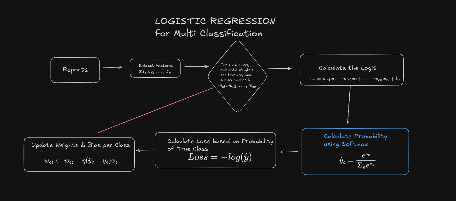
So the softmax replaces only the sigmoid. Everything after it stays: the loss is still minus the log of the probability given to the true class (Section 4.1), and the weight update still has the form error times feature value. The chart sets the two cases side by side; the three-class column uses made-up logits for three cancer types. Section C.1.4 derives the update rule in the last row.
Logits
One logit for the whole report
\(z = \mathbf{w}\cdot\mathbf{x} + b\)
Review 1: \(z = 0.90\)
One logit per class \(c\), each with its own weights
\(z_c = \mathbf{w}_c\cdot\mathbf{x} + b_c\)
Breast, Kidney, Lung: \(z = [2.0,\ 1.0,\ 0.1]\)
Step 1: logits become probabilities
Sigmoid
\(\hat{y} = \sigma(z) = \dfrac{1}{1 + e^{-z}}\)
\(\hat{y} = 0.711\) for label 1, so \(1 - \hat{y} = 0.289\) for label 0
Softmax
\(p_c = \dfrac{e^{z_c}}{\sum_k e^{z_k}}\)
\(p = [0.659,\ 0.242,\ 0.099]\)
Step 2: the loss
Minus the log of the probability of the true class
True label 1: \(L = -\log 0.711 = 0.341\)
Minus the log of the probability of the true class
True class Breast: \(L = -\log 0.659 = 0.417\)
The same rule in both columns. Only step 1 changed.
Step 3: the weight update
\(w_j \leftarrow w_j - \eta\,(\hat{y} - y)\,x_j\)
\(w_{c,j} \leftarrow w_{c,j} - \eta\,(p_c - y_c)\,x_j\)
\(y_c\) is 1 for the true class and 0 for the others
Put together, the whole process for many classes is the binary one of Figure 4.2 with the sigmoid swapped for the softmax:
4.2.2 Three classes: the six reports
Section 1.4.3 fitted logistic regression to the six toy pathology reports and noted that predict_proba turns three scores into three probabilities. Here is that claim checked by hand. First, the six reports and the fitted model:
The three logits are the weighted sums of Section 1.4.3 — the weights are in coef_, the biases in intercept_:
Now the softmax, by hand, next to scikit-learn’s answer:
Identical. predict_proba is one weighted sum per class and one softmax — nothing hidden.
The widget below starts from those three logits. Move them and watch the probabilities. Two things to try. Add 1 to every logit: the \(e^z\) column changes, but every probability stays exactly the same, because only the differences between logits matter. Then push one logit far above the others: its probability approaches 1 but never quite gets there. Underneath, the two-class case shows the softmax and the sigmoid giving the same number for any \(z\).
4.3 Keeping the weights in check: regularization
Fitting means choosing the weights \(w_{c,j}\) and biases \(b_c\). The criterion: make the training labels as probable as possible. Every candidate set of weights gives each training report \(i\) some probability \(P(y_i\mid x_i)\) for its correct label; good weights make all of those large. Taking logarithms and flipping the sign turns “make large” into “make small” — and gives the cross-entropy loss again, summed over the training reports. scikit-learn minimizes that, plus one more term:
\[ \mathcal{L}(w) = -\sum_{i=1}^{n}\log P(y_i\mid x_i) \;+\; \frac{1}{2C}\sum_{c,j} w_{c,j}^{2}. \]
The second term is a penalty on large weights, and the four reviews showed why it is needed. When the training data can be separated perfectly — and six toy reports, or 38,026 word columns for 7,354 reports, easily can — the loss keeps shrinking as the weights grow, so without a penalty the weights run off towards infinity. The penalty charges for size, which stops that. This is called regularization. (It is the penalty switch in the gradient-descent widget above: with it on, the map gets a lowest point and the search stops there.) C sets the exchange rate: small C makes the penalty expensive and the weights timid; large C makes it cheap and the weights bold.
At C=0.01 the model is squeezed so hard it barely commits — close to one third each. At C=100 it is emphatic. The data did not change; only the price of confidence did. And C is a choice made before fitting, exactly like k in Section 2.4 — so on the real corpus it is chosen on the validation set.
4.4 Logistic regression on the real corpus
As in Chapter 2, the full corpus is too heavy for a browser page, so the real-corpus code is shown with its output; it runs as written in Google Colab. The split is the one by hospital from Section 3.6: 5,489 training reports from 411 hospitals, 1,865 validation reports from 137 others, and 2,169 test reports from another 138. No hospital appears in more than one pile, and the vocabulary is built from the training reports only. Keeping hospitals whole has a price, which Section 2.7.3 warned of: the types cannot be kept in exact proportion, and four rare types (CHOL, DLBC, KICH and TGCT) have no test reports at all.
for features in ["counts", "presence"]:
    for C in [0.01, 0.1, 1, 10, 100]:
        model = LogisticRegression(C=C, max_iter=3000).fit(X_train, train["cancer_type"])
        accuracy = (model.predict(X_val) == val["cancer_type"]).mean()
validation accuracy C = 0.01 0.1 1 10 100
word counts 0.695 0.725 0.744 0.756 0.759
word presence 0.674 0.755 0.783 0.773 0.748Word presence beats word counts, and a moderate penalty is best: C = 1. Refitted on training and validation together, and run on the test set once:
Test accuracy, logistic regression (presence, C = 1):                    0.846
Test accuracy, nearest neighbors (@sec-tok-scoreboard's best setting):    0.489
Baseline:                                                                 0.108
Eighty-five percent, against forty-nine for nearest neighbors on the very same test reports, all from hospitals neither method has seen. (The nearest-neighbor setting is the one Section 3.6 chose for new hospitals: word counts with stopwords removed. With plain word counts it scores 0.411.) Learning a weight for every word, for every cancer type, beats copying the label of the most similar report by a wide margin.
The two methods also spend their effort at opposite ends:
                         fit on 7,354 reports    predict 2,169 reports    keeps
logistic regression      5 seconds               0.01 seconds             32 × 38,026 weights
nearest neighbors        0.01 seconds            1 second                 all 7,354 reports
Logistic regression does its work once, ahead of time, and condenses the training reports into a table of weights; after that, predicting is one weighted sum per class. Nearest neighbors does no work ahead of time and pays for it at every prediction.
4.5 Beyond accuracy
Eighty-five percent is an average over the 28 cancer types in the test set, of very different sizes. Accuracy alone cannot say which types are handled well and which badly, or what kind of mistake is being made. For that there are three more measurements and one table.
4.5.1 Precision and recall
Take a small example: 20 reports — 10 breast, 6 kidney and 4 lung — and a classifier’s predictions for them.
Eighty-five percent. Now ask two different questions about one class — lung:
- Recall: of the reports that really are lung, what fraction did the classifier find? Two of the four: recall 0.5.
- Precision: of the reports the classifier called lung, what fraction really are? Both of the two: precision 1.0.
The lung predictions are trustworthy when they are made — but half the lung reports are missed. Kidney is the opposite: all six kidney reports are found (recall 1.0), but 9 reports were called kidney and only 6 are (precision 0.67), because the missed lung reports and one breast report were called kidney too. The two measurements catch different failures, and which one matters more depends on the use: a screening tool that must not miss a cancer needs high recall; a tool whose every alarm triggers an expensive follow-up needs high precision.
4.5.2 The confusion matrix
Both come from one table: true classes down the side, predicted classes across the top, and the count of reports in each combination.
The diagonal holds the correct predictions. Everything off the diagonal is a mistake, and its position says which mistake: two lung reports called kidney, one breast report called kidney. Recall for a class reads along its row (2 of the 4 lung reports are on the diagonal); precision reads down its column (6 of the 9 reports in the kidney column are kidney).
4.5.3 F1, and averaging over classes
A single number that balances the two is the F1 score, the harmonic mean of precision and recall:
\[ F_1 = \frac{2 \cdot \text{precision} \cdot \text{recall}}{\text{precision} + \text{recall}} . \]
It is high only when both are high — for lung, \(2 \cdot 1.0 \cdot 0.5 / 1.5 = 0.67\). scikit-learn prints all three for every class:
The last two rows average over the classes in two ways. The macro average treats every class equally, however small; the weighted average weights each class by its number of reports (the support column), so big classes dominate. With imbalanced classes the two can differ a lot, and the macro average is the one that notices when a small class is handled badly.
Try it in the widget below, which starts from the 20-report example. Click cells to make mistakes and watch which numbers move: a lung report called kidney lowers lung’s recall and kidney’s precision at the same time. Then load A rare class handled badly: 74 reports, of which only 4 are lung, and 3 of those 4 are called kidney. Accuracy is 96% and the weighted F1 is 0.95, yet lung’s F1 is 0.40, and only the macro average, 0.78, shows it.
4.5.4 The real report
On the real test set, for logistic regression and for nearest neighbors:
                       accuracy   macro F1   weighted F1
logistic regression      0.846      0.744       0.845
nearest neighbors        0.489      0.340       0.511
For logistic regression the macro F1 is well below the accuracy: several types do much worse than the average. Some of the weakest, with a few of the strongest for comparison:
| Cancer type | Test reports | Recall | Precision | F1 | Nearest neighbors’ F1 |
|---|---|---|---|---|---|
| Adrenocortical carcinoma (ACC) | 80 | 0.00 | 0.00 | 0.00 | 0.25 |
| Esophageal (ESCA) | 25 | 0.48 | 0.15 | 0.22 | 0.15 |
| Rectal adenocarcinoma (READ) | 4 | 1.00 | 0.16 | 0.28 | 0.00 |
| Lung squamous cell (LUSC) | 28 | 0.93 | 0.29 | 0.44 | 0.03 |
| Colon adenocarcinoma (COAD) | 60 | 0.68 | 0.67 | 0.68 | 0.16 |
| Stomach (STAD) | 157 | 0.58 | 0.89 | 0.70 | 0.11 |
| Lung adenocarcinoma (LUAD) | 165 | 0.66 | 0.93 | 0.77 | 0.17 |
| Breast (BRCA) | 217 | 1.00 | 0.88 | 0.93 | 0.95 |
| Thyroid (THCA) | 235 | 0.99 | 0.99 | 0.99 | 0.81 |
Most of the trouble is three pairs of neighboring types, and in each pair the mistakes run one way. The confusion matrix shows it:
                   predicted LUAD   predicted LUSC
true LUAD (lung, adeno)    109              54
true LUSC (lung, squamous)   2              26

                   predicted STAD   predicted ESCA
true STAD (stomach)         91              50
true ESCA (esophagus)       11              12

                   predicted COAD   predicted READ
true COAD (colon)           41              19
true READ (rectum)           0               4
(Each block shows only the two types of its pair, so a row can add up to less than its number of test reports.) The pairs are close in the body or in the tissue: two cancers of the same lung, told apart by cell type; stomach and esophagus, which meet at the gastroesophageal junction; colon and rectum, with the rectosigmoid junction literally between them. And the way the mistakes run explains the table’s odd mixture of numbers. Fifty-four lung adenocarcinomas called squamous cost LUAD a lot of recall, but they cost LUSC far more precision, because only 28 test reports are really squamous. Rectum is the extreme case: the model finds all 4 rectal reports, but it also calls 19 colon reports (and 2 others) rectal, so only 4 of its 25 “rectum” answers are right. A few mistakes from a big type can swamp a small type’s precision, which is the widget’s “rare class handled badly” in real data.
ACC is a different story. 80 of its 90 reports come from one hospital, and that hospital is in the test pile, so the model learned the type from 10 reports. It sends 30 of the 80 to the other adrenal tumor, pheochromocytoma (PCPG), and 11 to kidney clear cell (KIRC), from the neighboring organ; but it also sends 31 to breast, which no anatomy explains. Splitting by hospital is the honest test, and here it shows its price: when one hospital holds nearly all of a type, holding that hospital out leaves the type with almost nothing to learn from.
4.6 Confidence is not correctness
Logistic regression gives a probability with every prediction: the largest of the softmax outputs, the probability of the class it predicts. This is the model’s confidence, and it is tempting to read a high one as “probably right”.
The loss uses the probability of the true class, which is known only during training. The confidence uses the highest probability, which the model can give for any report, including a new one. When the prediction is right, the two are the same number; when it is wrong, the confidence belongs to a wrong class.
On the test set:
median probability of the predicted class, when right:    0.962
median probability of the predicted class, when wrong:    0.481
wrong predictions made with a probability above 0.9:      10% of all mistakes
The model is less sure of itself when it is wrong — useful — but about one mistake in ten comes with more than 90% confidence. A model’s probability is a statement about its own weights, not a guarantee about the world, and Section 1.4.3 already warned that it is not a clinical probability. Whether these probabilities can be trusted as probabilities is a question of calibration, and it returns in a later chapter.
Why confidence decides how the model can be used. In a hospital or a cancer registry, a classifier like this would not replace the people who read pathology reports; it would take part of the reading off their hands. So the practical question is not “how accurate is the model?” but “which reports can it be trusted with?” For a new report there is no true label to check against, and the model’s confidence is the only signal it gives, so confidence is what decides which reports the model keeps and which go to a person. Choosing a threshold weighs two costs against each other: the mistakes that get through unchecked, and the hours people spend on the reports the model passes on. A confident model can still be wrong, and its probabilities are not calibrated. So the threshold has to be chosen by testing it on reports whose labels are known, as the widget below does, not by assuming that 0.98 means right 98% of the time.
Even so, the probability can be put to work. Suppose the model answers only when its probability is above a threshold, and every other report is classified by hand, by a pathologist or a cancer registrar, as if there were no model. The widget below does this with the real test predictions. At a threshold of 0.9 the model answers 58.4% of the reports and is right on 97.5% of them, but 32 of its 335 mistakes still get through, because they were made with high confidence. Raising the threshold trades mistakes for work: at 0.99 the model answers only 24% of the reports, and passes on many it would have got right. No threshold on the slider removes every mistake; the most confident one, a colon report called rectal, was made with a probability of 0.9997.
4.7 What the model learned
Because the score is a weighted sum, the weights can be read: a large positive \(w_{c,j}\) means word \(j\) pushes a report toward type \(c\), a large negative one pushes it away. These are the biggest weights for some of the types that are hard to tell apart:
KIRC (clear cell)   +  clear, kidney, renal, conventional, fuhrman, cell
                    −  papillary, chromophobe
KIRP (papillary)    +  papillary, renal, cell, kidney, carcinoma, 8260
                    −  clear, chromophobe, conventional
LUAD (adeno)        +  adenocarcinoma, lung, lobe, nos, pleura, 03
                    −  squamous, cell
LUSC (squamous)     +  squamous, lung, cell, upper, lobe, lower
                    −  adenocarcinoma, 03
READ (rectum)       +  rectum, rectal, perirectal, rectosigmoid, adenocarcinoma, g2, ro
                    −  right, small, sigmoid, hemicolectomy
COAD (colon)        +  colon, sigmoid, hemicolectomy, adenocarcinoma, r0, pericolic
                    −  rectal, rectum, perirectal, rectosigmoid
Most of this is pathology a medical student would recognize. Each kidney type is pushed toward its own subtype’s name and away from the other two — “clear” counts against papillary, “papillary” against clear cell. The two lung cancers are each other’s mirror image. The colon and rectum lists are anatomy: where in the bowel the tumor sat, and which operation removed it.
Look closer, and the lists also show where the words come from:
- 8260 is part of “ICD-O-Code: 8260/3”, the standard diagnosis code for papillary carcinoma, which some hospitals print in the report. The model has learned to read the answer when it is written down as a number.
- ro is “R0” — no tumor left at the cut edge — with the zero misread as a letter by the scanner. The model learned a scanning error, because the error is consistent.
- g2 is “G2”, tumor grade 2 written as a code, as in “Adenocarcinoma tubulare (G2)”. The grade is real pathology, but this way of writing it belongs to a few hospitals’ templates: half of the rectal training reports contain it, and all of them come from just four hospitals. It marks who wrote the report as much as what it describes. (nos, “not otherwise specified”, as in “Adenocarcinoma, NOS”, is similar: standard wording that some hospitals use far more than others.)
- 03 is a plain number. It appears in only 37 training reports, as a fragment of measurements (“0.4 x 03 x 02 cm”) and of form fields, yet it weighs for lung adenocarcinoma and against squamous — noise the model has picked up because, in those few reports, it happened to line up with the label. Chapter 3 discussed what numbers do to a vocabulary.
The widget below shows these weights at work on a report, for the hardest pair. For each word it uses the word’s colon weight minus its rectum weight: how far the word tips the balance between those two types (the other 30 types are left out). Words that push toward colon are shaded blue, toward rectum orange, with the push written beside each word. The features are word presence, so a word counts once however often it appears. Load the examples, then edit the text. In the rectum report, change (Ro) to (R0): the scanning error and its correct spelling push in opposite directions. In the in-between report, delete Sigmoid colon and. Notice too the small pushes from words that say nothing about anatomy, such as and and free.
(To keep the page small, the widget keeps the 1,500 words with the largest pushes and treats the rest as zero. On the 64 colon and rectum reports in the test set, that changes the verdict for three.)
None of these is wrong to use, but each is a reminder that a weight records what predicts the label in the training reports. It does not establish a medical relationship, and words that mark a hospital or a scanner stop working the moment the reports come from somewhere else. That is why every score in this chapter comes from hospitals the model has never seen — and it raises the opposite question: how much better would the model look on hospitals it had seen?
4.8 Hospitals it has never seen
Section 2.7 found that nearest neighbors mostly matched reports by hospital template, and fell from 85% to 41% when the test reports came from hospitals it had never seen. That is why every split in this chapter keeps each hospital whole. The opposite experiment shows what knowing the hospital is worth: the same two methods, the same settings, on Section 2.4’s split made report by report, where nearly every test hospital also has reports in training:
                          seen hospitals    unseen hospitals
                          (Chapter 2's      (this chapter's
                          split)            split)
logistic regression           0.964              0.846
nearest neighbors             0.870              0.489
Logistic regression loses about twelve points; nearest neighbors loses nearly half of what it had. (Both nearest-neighbor figures use word counts with stopwords removed, Section 3.6’s choice for new hospitals.) The difference is in what each method can learn. Nearest neighbors compares whole reports, and whole reports from one hospital resemble each other in everything — headings, stock phrases, layout. Logistic regression learns one weight per word, shared across every report. A word that appears only in one hospital’s template helps with that hospital’s reports and no others, while a word like papillary helps with every papillary report from every hospital — so the weights end up dominated by the words of the disease. Twelve points is still a real loss, and Section 2.7’s lesson stands: quote the number measured under the conditions of real use. For a model meant for new hospitals, that is the 84.6%, not the 96.4%.
4.9 Nearest neighbors or logistic regression?
| Nearest neighbors | Logistic regression | |
|---|---|---|
| What it learns | nothing — it stores the training reports | one weight per word per type |
| Fitting | instant | seconds to minutes |
| Predicting | compares with every stored report | one weighted sum per type |
| Explains a prediction by | the reports it copied from | the words that pushed hardest |
| Test accuracy, new hospitals | 48.9% | 84.6% |
| Macro F1, new hospitals | 0.340 | 0.744 |
| Test accuracy, hospitals seen in training | 87.0% | 96.4% |
| Boundary | bends around the examples | straight |
The straight boundary turns out to be a strength here. With tens of thousands of word columns and a few thousand reports, there is room for a straight boundary to separate the types well — and a method that cannot bend around individual reports cannot memorize their quirks either. Nearest neighbors remains the better tool for one job: finding the reports most similar to a given one, which is search rather than classification, and which returns later in the book.
4.10 Summary
- A classifier learns its weights by minimizing a loss. For logistic regression it is the cross-entropy: the negative log of the probability given to the right answer, which rewards confident correct predictions and punishes confident wrong ones.
- Gradient descent improves the weights step by step; for each weight the step is the prediction error times the feature’s value. scikit-learn’s
fitruns a refined version of it. - With more than two classes, one logit per class becomes a probability through the softmax, of which the sigmoid is the two-class case.
- Regularization penalizes large weights, so they stay finite when the data can be separated perfectly. Its strength,
C, is chosen on the validation set. - On the real corpus, with every test report from a hospital it has never seen, logistic regression reaches 84.6%, against 48.9% for nearest neighbors and a baseline of 10.8%. On hospitals it has seen it would score 96.4%: the difference is what knowing a hospital’s template is worth, and it is not available in real use.
- Accuracy is not enough. Precision, recall and F1, per class and macro-averaged, and the confusion matrix show which types fail and how. The hardest pairs are neighbors in the body: lung adenocarcinoma versus squamous, stomach versus esophagus, colon versus rectum. A few mistakes from a big type can swamp a small type’s precision.
- A model’s probability is not its correctness, and its weights record what predicts the label in the training reports — including codes, scanning errors and template words.
Logistic regression has used the words exactly as CountVectorizer splits them, and counted every word alike. The next chapter improves how reports become numbers — weighting words by how informative they are, word pairs with a model that can weight them, and features built from what Chapter 3 found — and the chapter after it brings in other kinds of model, for a fair comparison side by side.