Appendix B — NumPy, pandas, and Data Wrangling

Appendix A covered the language. This covers the two libraries that nearly all practical NLP work is written with: NumPy and pandas.

Figure B.1: The four data structures this appendix is about, and how each one is built on the one below it. A Python list becomes a NumPy array, a NumPy array becomes a pandas Series, and aligned Series become a DataFrame — each layer adding structure, labels, and functionality.

ImportantThese code cells are live

Cells run in your browser and share one Python session, so run them in order from the top. If a cell reports that a name is not defined, you skipped one above it.

The first run takes fifteen to thirty seconds while Python, pandas, NumPy and matplotlib download.

B.1 NumPy

NumPy is one of the most important numerical computing libraries in Python. It provides fast and efficient tools for working with large collections of numbers, which makes it especially relevant to machine learning and NLP. Although text begins as strings, NLP models ultimately need numerical representations such as word counts, vectors, embeddings, and matrices. NumPy provides the underlying structures and mathematical operations needed to work with this numerical data efficiently. Many other popular libraries, including Pandas, scikit-learn, and parts of the scientific Python ecosystem, are built on or closely integrated with NumPy.

The central NumPy object is the NumPy array, or ndarray. Unlike ordinary Python lists, NumPy arrays are designed primarily for numerical data and usually contain values of the same type, allowing calculations to be performed much faster and more compactly. Arrays can also naturally represent one-dimensional vectors, two-dimensional matrices, and higher-dimensional data. This makes them well suited for representing NLP features such as document vectors or embedding matrices. NumPy arrays also provide an important bridge to Pandas, where objects such as a Series can be thought of as labeled one-dimensional arrays and a DataFrame as a labeled two-dimensional table built for more structured data analysis.

B.1.1 Arrays versus lists

How the code works:

• import numpy as np is universal convention. Essentially all Python code writes np..
• .shape is a tuple. For a one-dimensional array it reads (4,).
• counts * 2 multiplies every element. A plain Python list would repeat itself instead — try [525, 1034] * 2 and see.

B.1.2 Functions over a whole array

B.1.3 The top-N idiom

This deserves its own heading. It is how you answer “which words matter most to this model”, and it is not obvious.

np.argsort() returns the indices that would sort an array, not the sorted values themselves. For example, if weights = [2.10, 1.85, 0.02, 0.94, 1.40], then np.argsort(weights) returns [2, 3, 4, 1, 0]. The first number, 2, means that the smallest value is located at index 2, where the value is 0.02. The final 0 means that the largest value, 2.10, is located at index 0. This is useful because the same indices can then be used to reorder related arrays, such as the corresponding words in an NLP example.

How the code works:

• np.argsort returns the indices that would sort the array, ascending.
• Taking the last three, [-3:], therefore gives the three largest — but still in ascending order, so a bar chart drawn straight from it reads smallest-first. Reverse with [::-1] if you want the largest at the top.
• words[top_3] is fancy indexing: passing an array of positions to pull out several items at once. A plain Python list cannot do this.

That is the NumPy you need for now. Next we give those numbers labels.

B.2 From arrays to Series

A NumPy array holds values in order, and you reach them by position: counts[0], counts[1]. That is fine for pure numbers, but it forgets what the numbers are.

A pandas Series is the missing half: the same one-dimensional block of values, with a label attached to each one.

B.2.1 A Series is a labelled array

Figure B.2: The Series built in the cell below: four values, each addressed by a string label rather than by position. The index is ordered, the values stay a NumPy array underneath, and arithmetic applies to all of them at once — which is where a Series parts company with a plain dictionary.

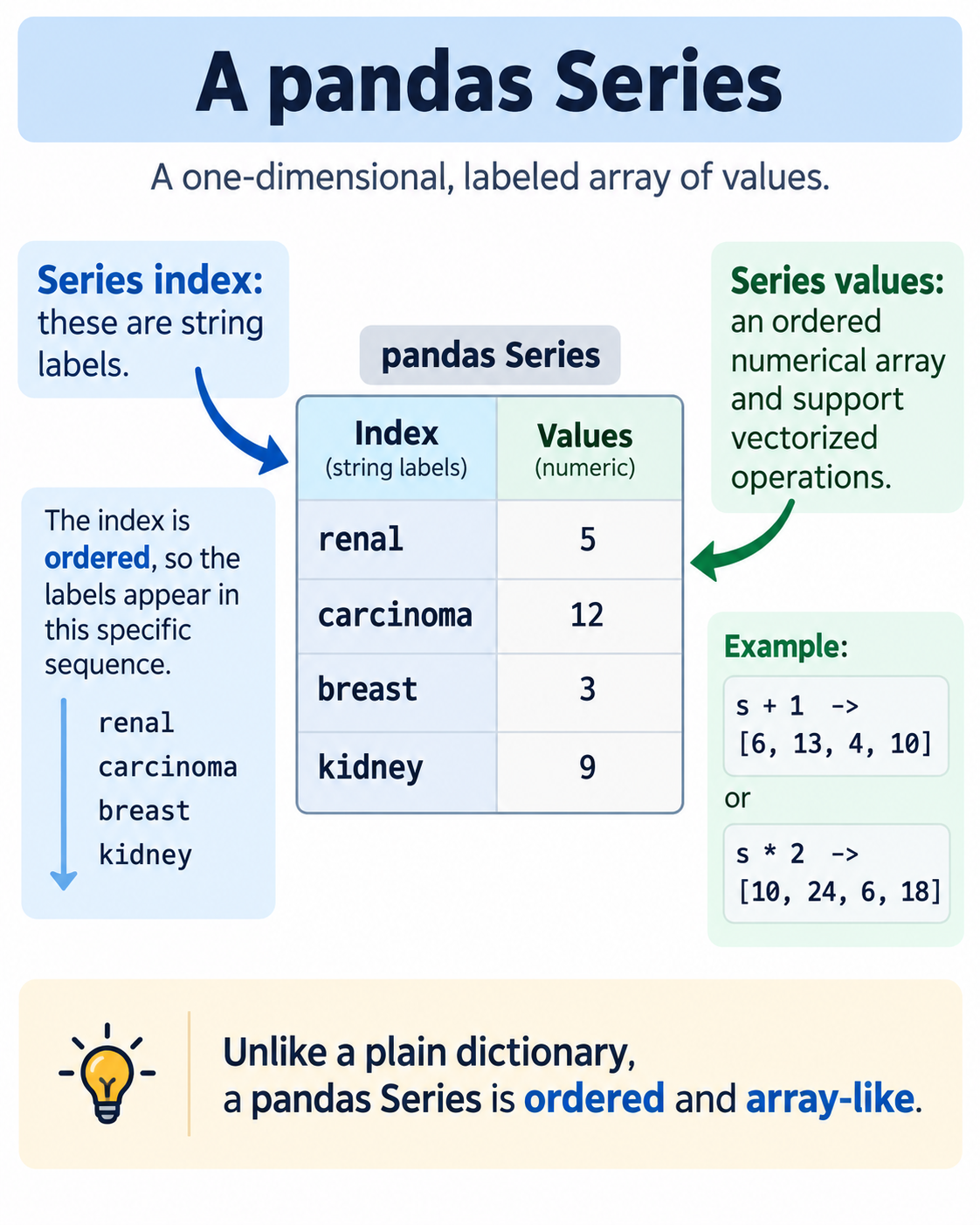
How the code works:

• pd.Series(values, index=labels) pairs each value with a label.
• Printing shows two columns: the index on the left, the values on the right. The index is not data — it is how you address the data.
• counts["breast"] looks a value up by name. The array could only do raw[2], and you had to remember what position 2 meant.
• That lookup reads exactly like a dictionary from Appendix A, and the resemblance is real — pd.Series(d) builds a Series from a dict, and counts.to_dict() goes back. The difference is what else a Series can do. counts * 2, counts.mean() and counts[counts > 4] act on the whole thing at once; a dict has to be walked one key at a time with a loop.
• A dict is a bag of keys. A Series is still a sequence, so the position survives alongside the label: counts.iloc[2] reaches the third value and counts[:2] slices the first two. The label is an addition to the position, not a replacement for it.
• Dict keys must be unique; Series labels need not be. That is a convenience until it is a bug, which is why the joins later in this appendix check .duplicated().any() first.

The values are still a NumPy array underneath:

So a Series is a NumPy array plus an index. Everything NumPy could do, it can still do.

B.2.2 The index

The word index means something different in NumPy and in pandas, and the difference is worth pinning down now, because it comes back at every level of this appendix.

A NumPy array has an index in the way a street has house numbers: positions 0, 1, 2, … that are implied by the order, cannot be changed, and carry no meaning of their own.

A pandas Series has a real index — an object in its own right, holding one label per value. You choose the labels. They can be text, they can be dates, they need not be in any particular order, and they can even repeat.

How the code works:

• The array has no .index at all. Position is the only way in.
• labelled.index is a pandas Index object — a labelled axis you can inspect, reuse, and match against.

Because the labels exist, a Series can be addressed two ways, and it is important to know which one you are using:

How the code works:

• .loc[...] always means label. .iloc[...] always means position.
• Bare labelled[...] guesses, and its guess depends on what the index contains. With text labels it looks up a label; with integer labels it looks up a label too, which surprises people who expected a position. When there is any doubt, say .loc or .iloc and the ambiguity disappears.

The labels are attached to the values, not to their positions. Reorder the Series and each value keeps its own label:

That is the property that makes the next section work, and the joins later on.

B.2.3 Series keep the NumPy behaviour

How the code works:

• Arithmetic applies to every value at once, exactly as with an array — but the labels come along for the ride.
• counts > 4 produces a Series of Booleans, and passing that back in keeps the rows where it is True. This is the boolean mask, and it is the workhorse of the rest of this appendix.

B.2.4 Labels line up automatically

This is the behaviour that makes Series worth having, and it has no equivalent in NumPy.

How the code works:

• The two Series list their words in different orders. Adding them still pairs renal with renal, because pandas matches on the label, not the position.
• Two NumPy arrays would have added position by position and produced nonsense, silently.

• Where a label is missing from one side you get NaN — “not a number”, pandas’ marker for absent data. It is a warning, not an error, and noticing it is your job.

This label-matching is the whole basis of joining tables later in Section B.7.

B.3 The DataFrame

A DataFrame is what you get when several Series share one index: a table with named columns and labelled rows. It is the object almost all data work in Python revolves around.

B.3.1 A DataFrame is a collection of Series

Figure B.3: The frame built in the cell below: three Series sharing one index, each becoming a named column. The columns hold different types — strings, integers, booleans — which is what separates a DataFrame from a two-dimensional NumPy array.

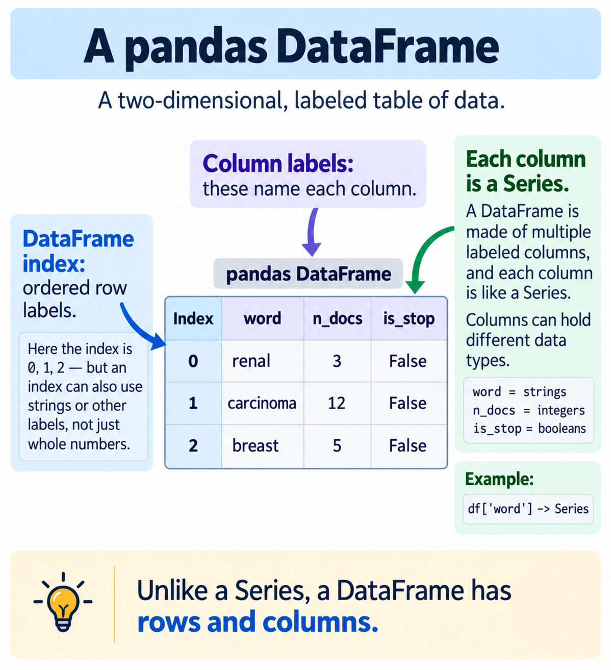
Build three Series, then put them side by side.

How the code works:

• Each key becomes a column name; each Series becomes that column.
• All three share the index 0, 1, 2, so their values line up into rows.
• The DataFrame’s index is that shared index — the row labels down the left.

And you can take a column back out, getting a Series again:

How the code works:

• vocab["n_docs"] returns a Series — the same object from before, index intact.
• Slicing a column out and putting one back are the two moves you will make most often.

B.3.2 The index again, one level up

The index you met for a Series is the same object here, doing the same job for a whole table. A DataFrame in fact has two of them: one labelling the rows, one labelling the columns.

How the code works:

• .index labels the rows, .columns labels the columns. Both are the same kind of pandas Index object.
• Column labels are usually text, which is why vocab["n_docs"] reads naturally. Row labels default to 0, 1, 2, … — which looks like NumPy positions but is not.

That last point is the trap. Default row labels happen to equal positions, so the distinction stays invisible until something disturbs it — and then it matters:

How the code works:

• Filtering kept rows 1 and 2 and threw away row 0. The labels came with the rows, so the index is now [1, 2] — it no longer counts from zero.
• tall.loc[1] returns the row labelled 1, which is the first row of the result. tall.iloc[1] returns the row in position 1, the second one. Different rows.
• The same .loc versus .iloc distinction as for a Series, and the same rule: say which one you mean.

Setting a meaningful index — patient identifiers, say, instead of 0, 1, 2 — is what makes rows addressable by name, and it is how two tables get joined in Section B.7.

B.3.3 Building one directly

In practice nobody makes the Series separately. You hand pd.DataFrame a dictionary of plain lists and it builds the Series for you.

How the code works:

• Each list becomes a column. Every list must be the same length.
• With no index given, pandas numbers the rows 0, 1, 2, 3.
• Writing the variable name alone on the last line displays it as a formatted table; print() gives cruder output.

B.3.4 A worked example

Something closer to real data: a handful of pathology-style reports, each with a label.

NoteA realistic shape, at a readable size

One row per document, one column of raw text, one column of labels. That is the shape almost every text-classification dataset arrives in, whatever the subject.

Real corpora run to thousands or millions of rows and are far too large to load in a browser, so six rows stand in here. Every operation below is exactly what you would run on the full thing.

B.3.5 Looking at it

How the code works:

• .shape is a tuple, so .shape[0] is the row count. You reach for it whenever you need to size something — a training split, say, as a fraction of the whole.
• .head() shows the first five rows by default. On a table with thousands of rows this is how you look at it without flooding the screen.

B.3.6 Other ways to build one

How the code works:

• Each dictionary is one row; the keys become the column names.
• If a dictionary is missing a key, that cell becomes NaN rather than failing.

B.4 Reading and writing CSV files

B.4.1 read_csv

How the code works:

• sep="," names the separator and header=0 says the first line holds column names. Both are the defaults, but stating them explicitly is a good habit: the moment a file breaks the convention you will already be looking in the right place.
• StringIO lets us treat text as a file, so these examples run in your browser. In real code the first argument is a path to a file on disk.

B.4.2 When the separator is not a comma

How the code works:

• Without sep=";" pandas finds no commas, so it reads each whole line as a single column. You get one column with a very long name and no error at all.
• This is a real file in the course data, and this is a real way to lose an hour.

B.4.3 Writing

How the code works:

• index=False stops pandas from writing the row labels as an extra unnamed first column. Pass it every time. Omit it once, read the file back, and you will find a mysterious Unnamed: 0 column that was not there before.

B.5 Selecting

B.5.1 Columns

How the code works:

• df["col"] gives one column as a Series.
• df[["a", "b"]] gives a DataFrame. The inner brackets are a list of column names — that is the whole reason for the doubling, and knowing that makes it stop looking arbitrary.

B.5.2 Getting plain Python back

How the code works:

• .values gives a NumPy array; .tolist() turns that into an ordinary list.
• You do this before handing text to scikit-learn, which wants a plain list of strings rather than a pandas object.

B.5.3 Filtering rows

How the code works:

• Comparing a column to a value gives a boolean mask — one True/False per row.
• Passing the mask back into df[...] keeps the True rows. Usually written in one line: reports[reports["cancer_type"] == "KIRC"].

B.5.4 isin and negation

How the code works:

• .isin([...]) tests against several values at once — the alternative to chaining or.
• ~ negates a mask. You must use ~, not not; not on a Series raises ValueError: The truth value of a Series is ambiguous, because Python does not know whether you mean “all of them” or “any of them”.

B.6 Creating and transforming columns

B.6.1 Assignment creates a column

How the code works:

• Assigning to a name that does not exist creates the column.
• .apply(func) runs a function on every value and collects the results. With a lambda this becomes a one-liner — the pattern from Appendix A, now doing real work.

Extracting an identifier from a filename column has exactly this shape:

B.6.2 Checking for duplicates

How the code works:

• .duplicated() marks each value True if it has been seen earlier, so the first occurrence is False.
• .any() collapses that to a single True/False, which is what you put in an assert.

B.6.3 Checking for missing values

How the code works:

• .isna() gives True wherever a value is missing. .notna() is its opposite.
• .sum() counts the Trues, because True counts as 1. So .isna().sum() is “how many missing”, in one step.
• On a whole DataFrame, .isna().sum() returns one count per column. This is the first thing worth running after a join: a column that was full before and has holes now tells you the join failed to find a match for those rows.
• .any().any() collapses twice — once down each column, then across columns — to a single True/False for the entire table.

To act on what you find: .dropna() removes rows with holes, and .fillna(value) replaces them. Neither is automatically right. A missing label usually means the row cannot be trained on; a missing count might legitimately be a zero.

B.6.4 copy, and the warning you will see

How the code works:

• Without .copy(), kidney may be a view onto reports, and assigning into it raises SettingWithCopyWarning — pandas warning that it cannot tell whether you meant to change the original.
• Rule of thumb: if you filter rows and then intend to modify the result, add .copy().

B.7 The index, and joining without merge

This is the hardest idea in this appendix, and the one that unlocks the most code.

B.7.1 Every DataFrame has an index

By default the index is 0, 1, 2… But it does not have to be.

B.7.2 Setting a meaningful index

How the code works:

• The index becomes the patient barcode, so a row can be fetched by name rather than by position.
• .loc[row_label, column_name] reads one cell.

B.7.3 .loc has two jobs

How the code works:

• Same accessor, two mental models: .loc[label, col] for a lookup, .loc[list] for row selection. The resemblance between the two confuses people, so it is worth pausing until the difference is clear.

B.7.4 The join

Now the payoff. Two tables, matched on patient barcode, without merge.

How the code works — slowly, because this line does a lot:

1. corpus.index is the list of barcodes we have reports for, in report order.
2. labels.loc[those_barcodes, "cancer_type"] pulls each patient’s label out of the second table, in the order asked for.
3. Assigning the result adds it as a column.

Three consequences worth noticing:

• Order does not matter. The labels table lists TCGA-A2-A0T2 first; the result still lines up correctly, because matching is by label, not by position.
• Extra rows are dropped silently. labels has five patients, corpus three. The two unmatched patients simply never appear. On the real data this is how 11,160 labels become 9,523 rows.
• A missing label would give NaN, not an error. Guard against it beforehand: assert corpus["patient_id"].isin(labels["patient_id"]).all().

B.7.5 The more usual way

Most pandas code you meet elsewhere uses merge.

How the code works:

• merge matches on a named column rather than on the index, and how="left" keeps every row of the left table.
• Same result here. merge is more explicit and more common; the index method is more compact and turns up constantly in text-processing code. Be able to read both.

B.8 Counting and summarising

B.8.1 value_counts

How the code works:

• .value_counts() counts each distinct value, largest first. This replaces the hand-written counting loop from Appendix A.
• normalize=True gives proportions instead of counts, which is how you check that a training split and a test split have similar class balance.

B.8.2 Chaining, and reading a chain

Read chains left to right: take the column, count the values, normalise them, turn the result into a dictionary. Four steps, one line. When a chain misbehaves, break it apart and print after each step.

B.8.3 describe and sort_values

How the code works:

• .describe() gives count, mean, standard deviation, min, quartiles and max in one call.
• .sort_values(by=...) sorts rows. ascending=True puts the worst first, which is usually what you want when hunting for problems.

B.8.4 Grouping

Every summary so far described a whole column at once. .groupby() splits the rows first, then summarises each group separately.

How the code works:

• .groupby("cancer_type") splits the table into one group per distinct cancer type. Nothing is computed yet.
• ["n_words"] picks the column to summarise, and .mean() computes it once per group. The result is a Series whose index is the group names.
• .size() counts the rows in each group. It answers the same question as value_counts() on that column, ordered by group name instead of by count.
• The result is an ordinary Series, so it chains: .sort_values() to rank the groups, .plot(kind="bar") to see them.

Read it as one sentence: split by cancer type, take the word counts, average them.

NoteWhy this matters for a classifier

Grouping a feature by the label is how you find out whether the feature gives the answer away. If median report length differs sharply between cancer types, then length alone carries information about the label — and a model that looks accurate may be reading document length rather than the words.

B.9 Plotting a DataFrame

How the code works:

• .plot(kind="bar") works straight off a Series or DataFrame.
• fig, ax = plt.subplots() makes a figure and axes; ax is what you label.
• Always label the axes. An unlabelled chart is a chart nobody can check, and a mislabelled one is worse than none at all.

B.9.1 Horizontal bars

barh is the usual shape for showing which words a model weighs most heavily. The words come from argsort over the coefficients and the inverted vocabulary dictionary from Appendix A.

B.10 Past the DataFrame

The last step of the pipeline hands your data to scikit-learn, and what comes back is not a table.

B.10.1 A sparse matrix

How the code works:

• .fit_transform returns a sparse matrix, not a DataFrame. It has .shape, but printing it lists coordinates rather than drawing a table.
• Sparse means only the non-zero entries are stored. On the real corpus the matrix is 4,761 by 23,818 — 113 million cells, almost all zero. Stored densely that is roughly a gigabyte; stored sparsely it is trivial.
• Code often names these variables something like arr_bow, which is misleading. It is not an array, and it will not behave like one.

B.10.2 Making it readable

How the code works:

• .toarray() expands the sparse matrix into a full NumPy array, which pandas can wrap.
• Fine for six documents. Never do this on the real corpus — that is the gigabyte.

B.10.3 The estimator protocol

Every scikit-learn object follows the same three-verb pattern.

How the code works:

• fit learns from data. transform converts data using what was learned. predict applies a fitted model to new input.
• fit_transform is just the two run together, and you call it only on training data.
• Attributes ending in an underscore — classes_, coef_, vocabulary_ — exist only after fitting. That trailing underscore is scikit-learn’s convention for “learned from your data”, and asking for one too early is a common error.

B.11 Exercises

B.11.1 Selecting and filtering

# 3. a boolean mask: df[df["n_words"] > 300]
# 4. .isin(["KIRC", "LUAD"])
# 5. ~ in front of the whole condition, not the word "not"

B.11.2 Making a new column

# .apply(lambda t: ...) runs a function on every value in the column.
# len(t.split()) counts words;  "carcinoma" in t  tests membership.

B.11.3 The index join

# df.index = df["patient_id"].values
# Then: docs["cancer_type"] = meta.loc[docs.index, "cancer_type"]
# For 4: compare len(meta) with len(docs).

B.11.4 Counting classes

# .value_counts() and .value_counts(normalize=True).round(3)
# A value_counts result is itself a Series, so you can filter it:
#     counts[counts < 4]

B.12 Summary

After this appendix you should be able to:

• NumPy — make an array, read its shape, apply arithmetic and functions to all of it at once, and use argsort()[-n:] with fancy indexing to pull out the top N.
• DataFrames — build one from a dictionary or a list of dictionaries, and inspect it with .shape, .head() and .columns.
• CSV — read with an explicit sep and header, recognise the damage a wrong separator does, and write with index=False.
• Selecting — single versus double brackets, .values.tolist() to get plain Python back, boolean masks, .isin(), and ~ for negation.
• Transforming — create columns by assignment, apply a lambda down a column, check .duplicated(), and know when .copy() is needed.
• The index — set it from a column, use both forms of .loc, and read the index-alignment join that some code uses in place of merge.
• Summarising — .value_counts() with and without normalize, .describe(), .sort_values(), and plotting the result.
• Handing off — recognise a sparse matrix, know why not to densify it, and follow the fit / transform / predict protocol and its trailing-underscore attributes.

That is the toolkit nearly every practical NLP workflow is built from.